WSN Profiler
Author: Josh Thomas
To obtain connectivity profiles for the wireless sensor network topologies used in our evaluation of CTP, we have adapted an application suite called TestbedProfiler initially developed by Chad Metcalfe, Tracy Camp, and Michael Colagrosso at Colorado School of Mines. This utility reveals the underlying connectivity of a wireless sensor network by systematically recording and then analyzing the reception of packets that are broadcast by each node in the network.
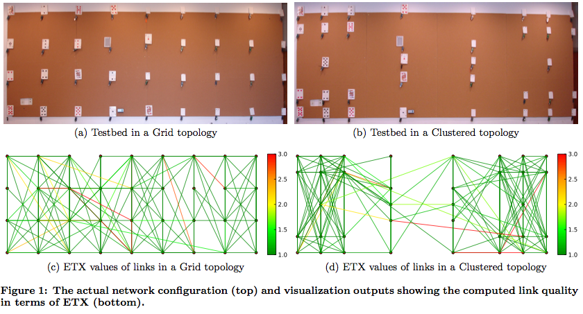
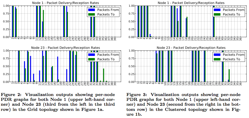
In its original form, TestbedProfiler provides a number of useful connectivity statistics, such as packet delivery ratio (PDR), average RSSI and LQI values, and average neighbor count. It also generates simple connectivity charts that indicate the presence or absence of connections between nodes–but not the quality of those connections. Seeing this as a limitation of a useful tool, we modified TestbedProfiler to produce two additional types of graphs. The first is a spatial representation of the network that shows connections between nodes in terms of their estimated transmission count (i.e., ETX), which is a measure of the quality of a connection (see Figure 1). The ETX of a link is the total number of packet transmissions and retransmissions required to send a packet back and forth across the link one time, assuming that each node in the route retransmits the packet until it is successfully received. The second type of graph is generated for each node and shows the PDR both to and from every other node in the network (see Figures 2 and 3).
Because we see this tool as being useful beyond the scope of simple testbed deployments, we refer to our enhanced version simply as `WSN Profiler’. In this section, we first provide a brief overview of its components and then describe each in detail.
TinyOS application: The TinyOS application runs on the node hardware itself. It transmits bursts of packets to elicit connectivity information from its neighbors, which, running the same code, report details of each packet they receive to a central server.
Profile Server: The Profile Server, which is linked to the nodes via a serial connection, controls the execution of the profile experiment. It tasks each node to begin its transmissions in turn and also logs incoming packet data for later processing.
Analysis and Visualization Scripts: These scripts are a collection of scripts that are run post-experiment on the resulting data to provide average statistics and a visualization of network connectivity.
TinyOS Application
As mentioned, TestbedProfiler makes use of a TinyOS application (TestbedProfilerC) that runs directly on the nodes that comprise the network in question. TestbedProfilerC has two context-dependent roles, which can be conceptualized as sender and receiver.
In its role as sender, the application lies dormant until it receives a command to broadcast, which comes in the form of a serial message from the profile server. Once instructed, the node broadcasts the specified number of packets at regular intervals using its radio and a simple periodic timer. The program is wired to the CC2420 radio stack, making it deployable only on nodes that utilize the CC2420 hardware.
TestbedProfilerC also functions passively as a receiver. When a node hears a broadcast packet sent from one of its neighbors, it reports reception of the message to the profile server. The report contains the sender’s ID, the recipient’s ID, the packet sequence number, and the RSSI and LQI values for the received message. Because the report is sent via the node’s serial connection to the profile server, it provides a reliable means of data delivery that does not interfere with the radio experimentation.
Profile Server
The Profile Server is a computer running TestbedProfiler–a command-line Java program responsible for controlling the execution of the experiment. It must be connected to all nodes that will be profiled via a serial connection (USB, for example).
Once run, the program has two main responsibilities. First, it must sequentially task each node to broadcast, ensuring that only one node is broadcasting at a given time. Second, it must listen for incoming packets from the nodes and write them to a trace file for later processing and analysis. Each packet reception event adds a single line–consisting of receiver ID, source ID, packet sequence number, RSSI, and LQI–to the trace file. The receiver ID is the ID of the node that received the packet; the source ID is that of the packet’s sender. The sequence number of the packet is simply a running zero-based count of the number of packets sent by the currently transmitting node. The RSSI and LQI values for the packet are retrieved directly from the receiving node’s radio hardware and provide a means to quantify the perceived strength of the reception event.
The Java interface has been updated to provide the user greater control over the details of the profile collection, allowing it to better reflect the WSN application he or she intends to deploy. The command to broadcast originally contained only the desired number of iterations and the power level at which to transmit; radio channel and message interval were hard-coded on the nodes to channel 15 and to 50ms, respectively, and packets of sizes 25, 50, 75, and 100 bytes were sent for each iteration. Now, however, the user is also able to specify the radio channel on which to broadcast, the interval between the transmission of one message to the next, and the size of the packet to be sent. Additionally, a single invocation of the profiler originally repeated the same procedure for a range of power levels, but now one invocation corresponds to one power level. This prevents the mingling of disparate data and simplifies automation (e.g. using shell scripting).
Analysis and Visualization Scripts
WSN Profiler includes a number of scripts that help make sense of the raw connectivity data gathered by the profile experiment. A pair of python scripts were included with the original version of TestbedProfiler?. The first, CreateProfile?, parses a data profile and calculates statistics for each node in the network. This includes a summary of its connectivity to other nodes with packet delivery rates, average RSSI and LQI values, and average neighbor count. The second script, CreateDigraph?, generates a simple connectivity graph that shows connections between nodes. However, this graph does not indicate the quality of the connections. This means that no distinction is made on the graph between a link in which 100% of packets were successfully delivered and one in which 0.01% of packets were delivered.
Aware that this is a significant limitation, we expanded the post-experiment output to include two additional graphs, both of which convey both quantity and quality of links. The first new type of graph (see Figures 1c and 1d) provides a 2-dimensional representation of nodes in the network and indicates connections by lines between nodes. The color of each line is based on the ETX of the link that line represents, normalized to the color scale shown on the right side of the graph. An ETX of one, represented by dark green, indicates a high-quality connection in which no packets are lost. Conversely, an ETX of infinity would represent the absence of a connection and is not shown. The user can specify the upper ETX limit of what is considered a true connection; we use an upper ETX ceiling of three, meaning that links with an ETX of more than three are not shown. This type of graph is excellent at quickly conveying the degree of connectivity in the entire network and for identifying potentially problematic links.
The second type of graph shows node-specific connectivity information and is automatically generated for every node in the network (see Figures 2 and 3). It shows both incoming and outgoing packet delivery ratios for the node relative to every other node in the network. A PDR of one for packets from the node to a second node indicates that the second node received every packet sent by the first; likewise, a PDR of one for packets to the node means that the node received every packet sent by the other. A PDR of zero, of course, means the opposite. These graphs are very useful in identifying how well a node is connected to the rest of the network, the quality of a specific link, and asymmetric (e.g. one-way) connections.